LCnetgen Example 5, Multi-Section LF Loading Coil
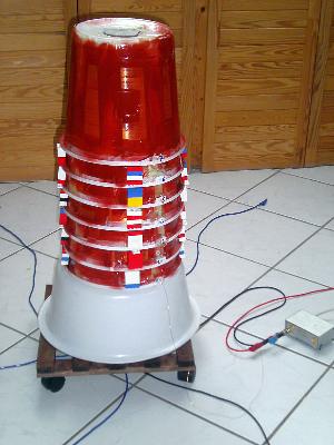 This coil, built and used by Markus Vester DF6NM, is made from seven
identical nested bucket coils as shown in the adjacent
photo. As you can imagine, the normal mode spectrum of this coil is quite
rich and it is a good test of LCnetgen to model it correctly.
This coil, built and used by Markus Vester DF6NM, is made from seven
identical nested bucket coils as shown in the adjacent
photo. As you can imagine, the normal mode spectrum of this coil is quite
rich and it is a good test of LCnetgen to model it correctly.
To achieve good accuracy for several of the lowest resonances requires
over 30,000 tiles and needs about 3.5 Gbyte of RAM and a few hours to run
using the current version of LCnetgen. This is entirely due to
the close proximity of the windings to each other. The mutual capacitance
between windings needs to be modelled quite accurately in order to obtain
correct predictions of the higher mode frequencies.
Input file
Input file
df6nm_coil.in
contains
   ;
   ; Dimensions of each bucket winding
   ;
   lower_diam = 0.254
   upper_diam = 0.211
   coil_length = 0.216
   coil_turns = 480
   wire_diam = 0.4e-3
   coil_sections = 9
   coil_tiles = 400

   ; Seven identical coils.
   ; Going from bottom to top of the stack, the six axial spacings between
   ; the beginnings of consecutive windings are 50, 53, 50, 53, 50, 50 mm.

   coil1_base = 0.25
   coil2_base = coil1_base + 50e-3
   coil3_base = coil2_base + 53e-3
   coil4_base = coil3_base + 50e-3
   coil5_base = coil4_base + 53e-3
   coil6_base = coil5_base + 50e-3
   coil7_base = coil6_base + 50e-3

   coil {
     name coil1
     end1 0, 0, coil1_base

     wirad wire_diam/2
     axis 0, 0
     length coil_length
     radius1 lower_diam/2
     radius2 upper_diam/2
     turns coil_turns
     sections coil_sections
     tiles coil_tiles
   }

   coil {
     name coil2
     end1 0, 0, coil2_base

     wirad wire_diam/2
     axis 0, 0
     length coil_length
     radius1 lower_diam/2
     radius2 upper_diam/2
     turns coil_turns
     sections coil_sections
     tiles coil_tiles
   }

   coil {
     name coil3
     end1 0, 0, coil3_base

     wirad wire_diam/2
     axis 0, 0
     length coil_length
     radius1 lower_diam/2
     radius2 upper_diam/2
     turns coil_turns
     sections coil_sections
     tiles coil_tiles
   }

   coil {
     name coil4
     end1 0, 0, coil4_base

     wirad wire_diam/2
     axis 0, 0
     length coil_length
     radius1 lower_diam/2
     radius2 upper_diam/2
     turns coil_turns
     sections coil_sections
     tiles coil_tiles
   }

   coil {
     name coil5
     end1 0, 0, coil5_base

     wirad wire_diam/2
     axis 0, 0
     length coil_length
     radius1 lower_diam/2
     radius2 upper_diam/2
     turns coil_turns
     sections coil_sections
     tiles coil_tiles
   }

   coil {
     name coil6
     end1 0, 0, coil6_base

     wirad wire_diam/2
     axis 0, 0
     length coil_length
     radius1 lower_diam/2
     radius2 upper_diam/2
     turns coil_turns
     sections coil_sections
     tiles coil_tiles
   }

   coil {
     name coil7
     end1 0, 0, coil7_base

     wirad wire_diam/2
     axis 0, 0
     length coil_length
     radius1 lower_diam/2
     radius2 upper_diam/2
     turns coil_turns
     sections coil_sections
     tiles coil_tiles
   }

   ;
   ;  Something to represent the surroundings.
   ;

   electrode {
      name ground

      disc {
         radius 3
         center 0, 0, 0
         axis 0, 0
         tiles 1000
      }

      cylinder {
         radius 3
         end1 0, 0, 0
         length 3
         axis 0, 0
         tiles 1000
      }

      disc {
         radius 3
         center 0, 0, 3
         axis 0, 0
         tiles 500
      }
   }
Generate a Spice sub-circuit with
lcng -o spice df6nm_coil
Test Circuit
In this test the base of the coil is driven with 1V AC and the drive
current is measured to produce an input admittance plot. The test circuit is
df6nm_coil-unloaded.spice
which contains
   df6nm_coil
   .OPTIONS NOMOD NOPAGE
   .AC LIN 10000 1K 1000K
   .PRINT AC V(J7) I(Vin)
   .INCLUDE df6nm_coil.spice

   * pin 1: zero of potential at infinity
   * pin 2: GROUND
   * pin 3: COIL7 end1, 0.00 turns
   * pin 4: COIL7 end2, 480.00 turns
   * pin 5: COIL6 end1, 0.00 turns
   * pin 6: COIL6 end2, 480.00 turns
   * pin 7: COIL5 end1, 0.00 turns
   * pin 8: COIL5 end2, 480.00 turns
   * pin 9: COIL4 end1, 0.00 turns
   * pin 10: COIL4 end2, 480.00 turns
   * pin 11: COIL3 end1, 0.00 turns
   * pin 12: COIL3 end2, 480.00 turns
   * pin 13: COIL2 end1, 0.00 turns
   * pin 14: COIL2 end2, 480.00 turns
   * pin 15: COIL1 end1, 0.00 turns
   * pin 16: COIL1 end2, 480.00 turns

   * J7 is the top terminal, J0 is the base terminal
   X1 0 0 J6 J7 J5 J6 J4 J5 J3 J4 J2 J3 J1 J2 J0 J1 df6nm_coil

   * Signal generator, 50 ohm output impedance
   Vin 1 0 DC 0 AC 1
   Rin 1 J0 50

   .END
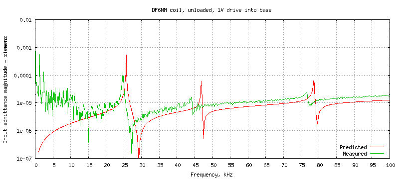
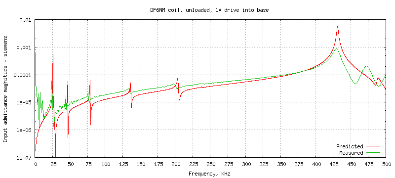
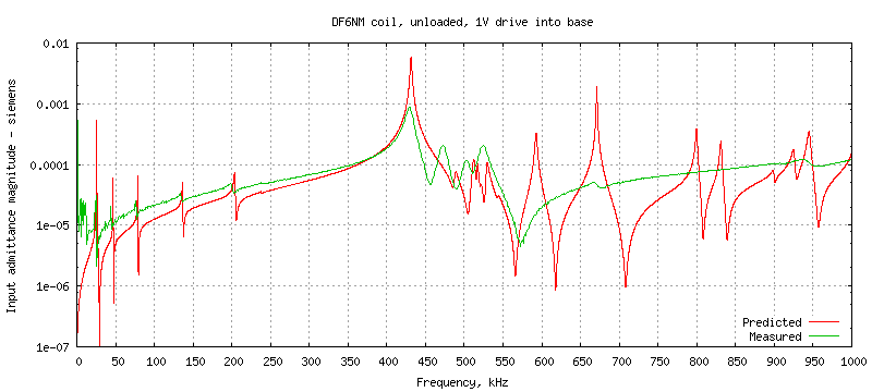
With one volt drive, the base current I(Vin) directly gives the input
admittance, which is plotted below for three frequency ranges:
The coil was also measured with a 270pF load capacitor to simulate the
typical antenna load. This is represented in the Spice test model by an
extra capacitance attached to the top of the coil,
CL J7 0 270e-12
and the comparison with the measured admittance of the loaded coil is
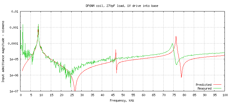
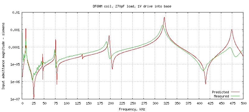
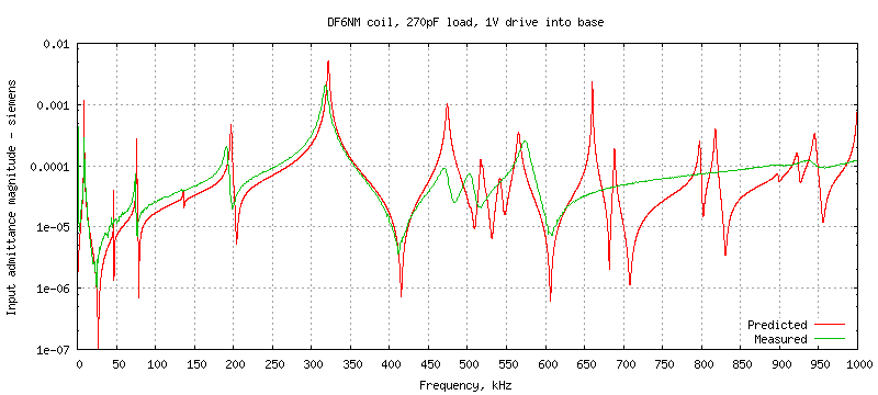
The predicted input admittance at the resonances is always higher in the model,
as are the corresponding Q factors. This is because lcng is only
using a simple model of AC resistance which takes approximate account of
skin depth but does not allow for proximity loss within the windings, which
is often quite significant. Also the model assumes lossless surroundings
intercepting the external E-field of the coil whereas in reality the return
current has to reach the signal generator via a complicated RC network formed
from walls, floor.
Time Domain
Spice can run a time domain simulation of the coil. A simple shell script can
gather the voltage measurements from Spice for each time step and produce
animations of the
resonances. Below is the voltage distribution of the 517kHz resonance
with a 1 volt AC drive into the base.
